
Database performance issues are a major contributor to the application slowdowns which we all face every day.
DBAs, developers and IT professionals have a daunting task of deciphering the large number of factors that contribute to database wait time. The challenge is both understanding how the database engine works and correlating it with other systems that support the application and the database.
Traditional database monitoring tools provides a simplistic view of health metrics and alerts that are unable to look at root cause or other factors outside the database that impact performance. The use of different tools to monitor each element of an application result in limited visibility and finger pointing.
Foglight’s SQL PI allows database experts and IT operations to take advantage of its Multi-Dimensional Performance Tree, to look across the application stack using many different dimensions. SQL PI gives visibility into root cause of performance issues very quickly. Figure 1 below, shows all the workload of an instance, the queries running including their context, resources being used and/or locked, and wait types encountered. In this 3 part series, we will walk through each of these 5 categories: workload, SQL Statements, context, resources and wait types - to see how easy it is to find the issue.
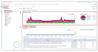
Figure 1
In just a few clicks, DBAs, Developers and IT operations can easily see what is impacting database response time in SQL PI. To find root cause however, you may need to know more about the issue. The 5 categories of dimensions in SQL PI can help guide you.
Dimension Categories
- Workload
SQL PI monitors the entire workload of the database instance. Figure 2 (below) shows the workload at the instance level for the last hour. Foglight keeps 13 months of performance data by default so it’s easy to compare today’s workload with that of yesterday, last week, or a specific timeframe in the past. From this view, you can see CPU Usage, the percent of Wait Time and the SQL average Response Time for the entire instance. Notice that the SQL average Response Time is over 7 seconds towards the end of the hour (figure 2). This was about the time the DBA got the call that things were slow. We can drill further into that specific timeframe to review.
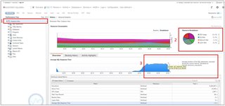
Figure 2
After drilling further in, we can see the SQL statement, ‘open getsumamount’ is taking 91 seconds for its average SQL Response time (figure 3). At this point we may want to review this SQL statement.
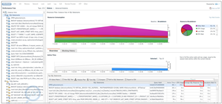
Figure 3
But first, a full review of the resources and wait types shows that the CPU usage is only at 15%, while the wait type, SOS SCHEDULER YIELD, accounts for almost 30% of total wait (see figure 4). Further investigation into this wait type might give more clues into fixing this issue - https://www.sqlshack.com/how-to-handle-excessive-sos_scheduler_yield-wait-type-values-in-sql-server/
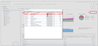
Figure 4
It should be noted, that in SQL PI, you don’t have to focus on the entire workload. If you know what resource is encountering a bottleneck, focus on that resource (in the second menu) to filter queries and other dimensions by that resource. Figure 5 shows how to find the most intensive CPU query in this instance.
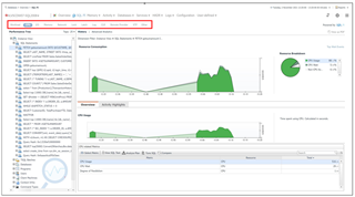
Figure 5
2. SQL Statements
There are many factors that impact SQL performance including number of executions, plans, and locking/blocking. Monitoring development environments enables proactive troubleshooting, but to truly understand SQL performance, developers need to have visibility into how their code works in production.
Foglight for databases is an agentless solution that puts minimal load on production server (less than 1 or 2%). To ensure the security of production performance data, Foglight has security settings, Active Directory integration provides multi-level permissions, and group / role based policies.
In our workload example, we found a SQL Statement, ‘open getsumamount’, that had very slow response time. It was coming from a TSQL Batch called 'dbo.GET_SUM_AMOUNT;1' which was spending 910.87 seconds (15+ minutes) on average for response time.
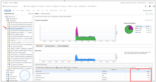
Figure 6
In Figure 6, we look at the TSQL Batch, to get the SQL text and the execution plan in Figure 7. SQL PI performs further analysis on expensive operators and objects in the execution plan and presents the plan in tabular format. You can always get the graphical execution plan by selecting the ‘open in SSMS’ button at the upper right corner. Additionally, you can see that this query had an execution plan change because the 'Compare Plans' button is highlighted.
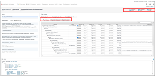
Figure 7
You can further examine the performance impact of this plan change by comparing the differences in workload on the 'Advanced Analytics' menu. Notice in Figure 8, the workload has increased significantly after the plan change.
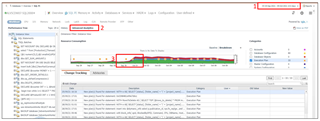
Figure 8
This concludes Part 1 of the Multi-dimensional Performance Analysis Series where we covered Workload and SQL Statement categories. Stay tuned for Part 2 where we will talk about further tuning SQL Statements and using 'Context' dimensions to drive to root cause.
